Finding a picture in an image without marking it up?

*We often see pictures in images: comics, for example, combine several pictures into one. And if you have an entertainment app where people post memes, like in our iFunny, you’re going to run into that all the time. Neural networks are already capable of finding animals, people, or other objects, but what if we need to find but another image in the image? Let’s take a closer look at our algorithm so that you can test it with a notebook in Google Colaboratory and even implement it in your project.* 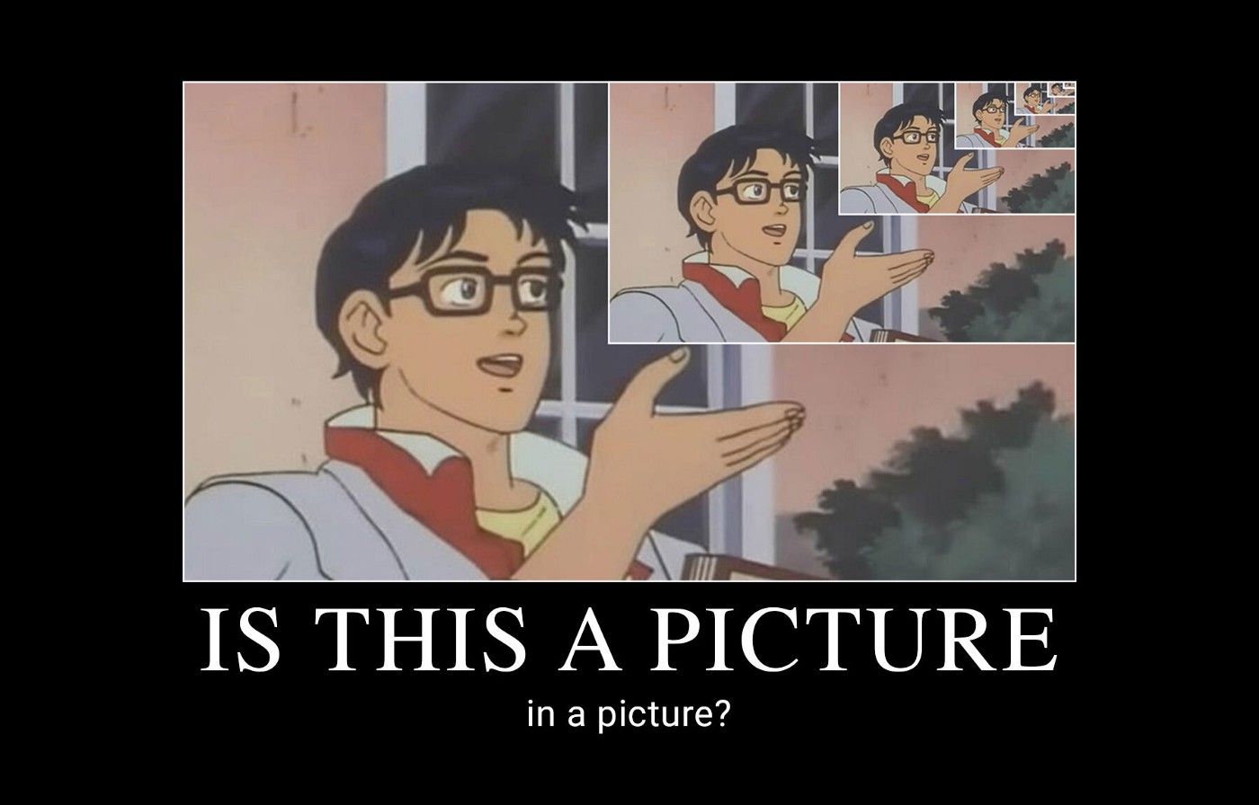  So, memes. Many of them consist of a picture and its caption, with the former serving as the context to the verbal joke: A meme can include several images with text:  One of the popular types of memes is screenshots of social network posts e.g. from Twitter. The picture occupies a relatively small area in them. Initially, the task of finding a picture in the image came up when we were sending push notifications. Before the advent of full-page push messages on Android, all the pictures in such messages were very small. The text was unreadable (Why would the user need it then?), and all the objects in the notification image were hardly informative. They were also less attractive. We decided to bet on pictures from memes. To increase the visual part, we made an algorithm that cuts out all the frames around the image, regardless of what is shown on it. **Let’s see the algorithm in action on a few examples (details below)** 1. Here’s how the algorithm handled the black background and the app watermark: 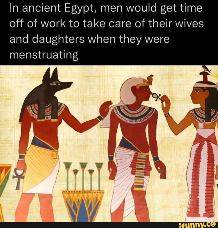*Before* *After* 2. In the following example, it did not separate the images, even though there was a large line between them. *Before* 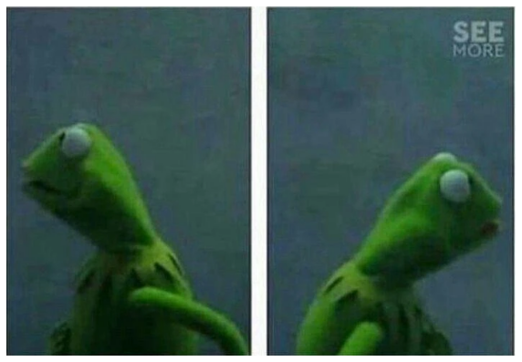*After* 3. This method is also suitable for large vertical text, which occupies about 50% of the area of the entire image. However, the algorithm missed the application watermark (there is still work to be done).  *Before*  *After* 4. The algorithm handled the following example with flying colors, even though the desired image occupied a relatively small percentage of the meme. The algorithm also trimmed the white frames on the sides. *Before* 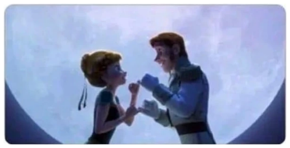*After* 5. In the next example, there were two backgrounds at once (white and black), but the algorithm coped with this. However, it left the white frames on the sides. *Before* 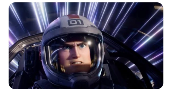*After* 6. The last example is particularly interesting because the image itself contains many lines. But even this did not confuse our algorithm. The upper boundary is a little bigger than we wanted it to be, but it’s a great result for such a difficult case! 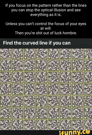*Before* 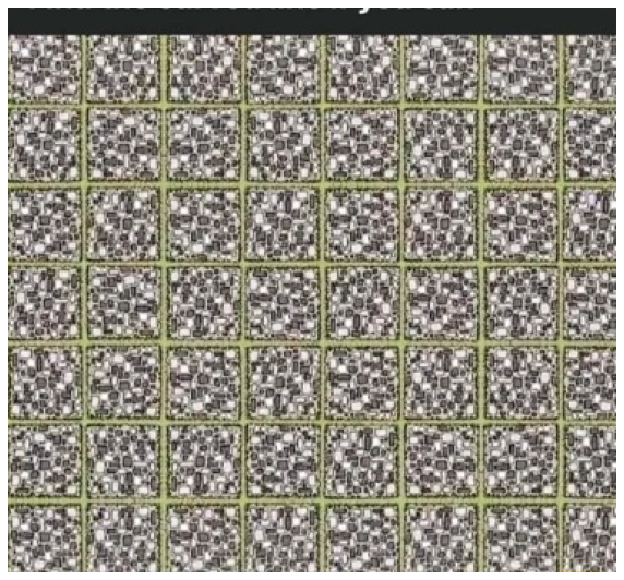*After* Recall that it was possible to achieve these results without markup. **The Algorithm** Let’s skip the uninformative parts of the code. You can find and run them yourself in the full [implementation](https://colab.research.google.com/drive/1u42OGNz4OEZCb7RakFhw6TETWpLCG3sb?usp=sharing) of the algorithm. In this article, we will focus only on the main idea. Let’s take this image with the puppies as an example. It has text at the top and a small strip of white background along with a watermark of our application at the bottom. 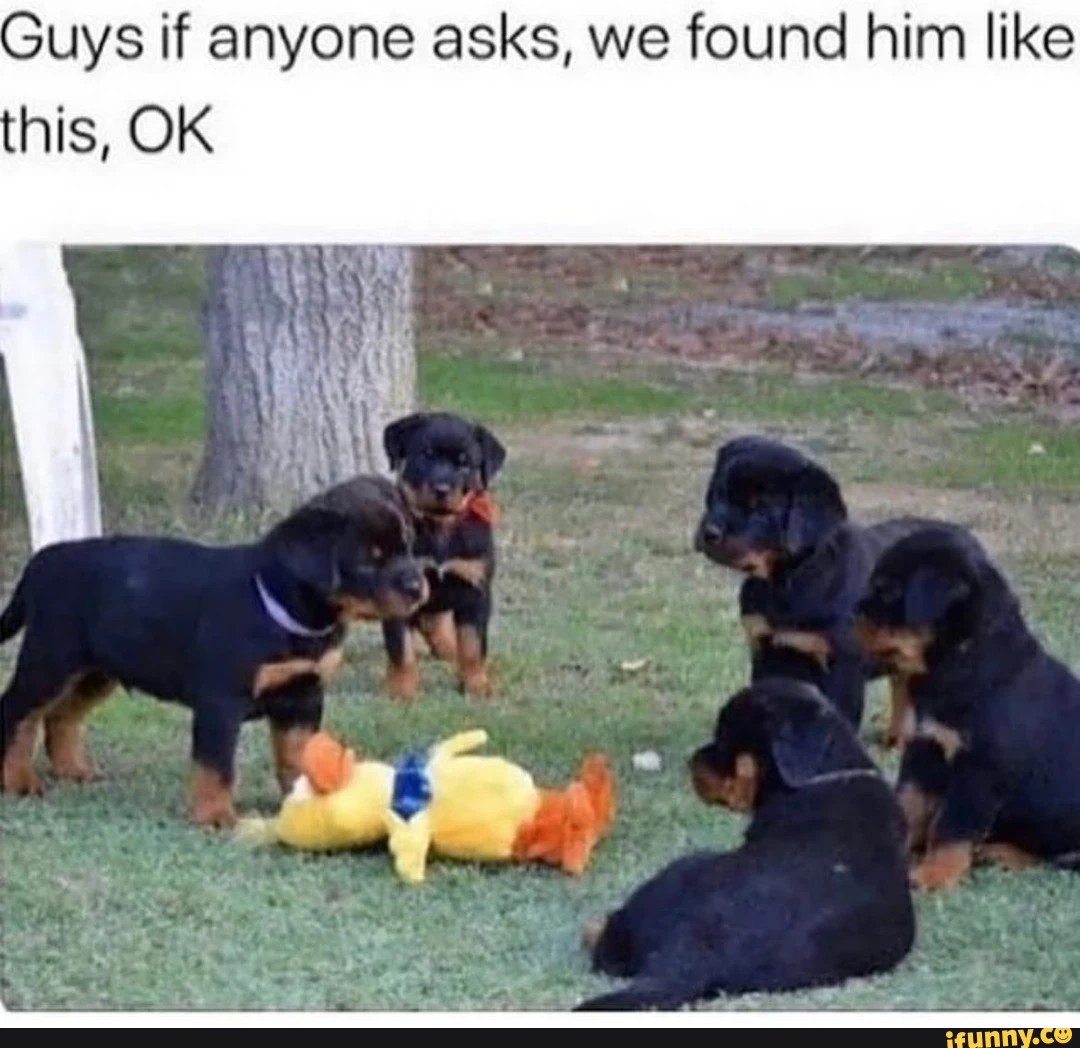To get just the picture with the puppies, we need to remove the two horizontal rectangles at the bottom and top. The basic idea is to recognize all the straight lines with the image using [the Hough Transform](https://en.wikipedia.org/wiki/Hough_transform) and then select those that border a white or black monotone area, which we will consider the background. **Step 1. Conversion of the image to Grayscale** The first step of image processing here is converting it to a monochrome format. There are many ways to do this, but I prefer getting the L-channel (lightness) in the [Lab](https://en.wikipedia.org/wiki/CIELAB_color_space) color space. This approach has proven to be the best in most cases. But you can try other approaches, say the V-channel (value) of the [HSV](https://en.wikipedia.org/wiki/HSL_and_HSV) color space. To eliminate the sharp contrast differences that create unnecessary lines in the image, we apply the Gaussian filter to the resulting black-and-white image. ``` img_gray = cv2.cvtColor(img, cv2.COLOR_RGB2LAB)[:, :, 0] img_blur = cv2.GaussianBlur(img_gray, (9, 9), 0) ``` Here we used functions from the OpenCV library. In addition to the image, the cv2.GaussianBlur function accepts the Gaussian kernel size (width, height) and the standard deviation along the X axis (along the Y axis, it is 0 by default). When using 0 as the standard deviation, it is [calculated ](https://docs.opencv.org/4.x/d4/d86/group__imgproc__filter.html#gac05a120c1ae92a6060dd0db190a61afa)based on the size of the kernel. The parameters we use are based on subjective experience. 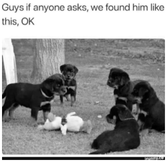*This is what we get at this point* You can find and use similar methods from the [scikit-image](https://scikit-image.org/) library, but be careful, as they differ in both results and input parameters. The Lightness channel of the [skimage.color.rgb2lab](https://scikit-image.org/docs/stable/api/skimage.color.html#skimage.color.rgb2lab) function result is in the range [0,100], and the Gaussian filter [skimage.filters.gaussian](https://scikit-image.org/docs/stable/api/skimage.filters.html#skimage.filters.gaussian) is more sensitive to kernel parameters. This affects the end result. **Step 2. Detecting edges** The Hough Transform, which is the basis of our algorithm, can only work with binary images that consist of a background and edges taking the values 0 and 1. We use [the Canny Transform](https://opencv24-python-tutorials.readthedocs.io/en/latest/py_tutorials/py_imgproc/py_canny/py_canny.html) to create a binary image. In short, this algorithm calculates the gradient in the intensity function of the pixel coordinate and finds its local maxima, the areas of which are defined as the desired edge. 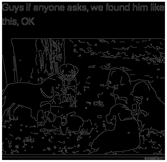*Result of the Transform* We use the Canny function of the Feature module from the [scikit-image](https://scikit-image.org/) library to perform the transform. You can find a similar function in the OpenCV library, but its implementation includes a 5x5 Gaussian filter smoothing, which makes it a bit difficult to control the situation. **Step 3. The Hough Transform** Now we need to detect the straight lines among all the lines we have found. Hough’s straight line transformation excels at this task. The algorithm draws a line at a given distance ρ from the origin and a certain angle θ to the X-axis, as shown below. 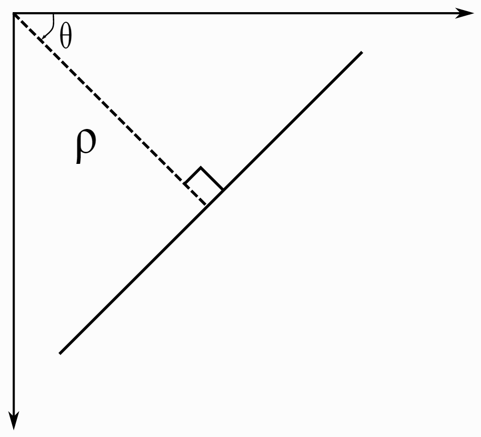For each such line, it calculates the number of the binary image light pixels that lie on the drawn line. The procedure is repeated for all ρ and θ values in the selected range. The result is an intensity map in (θ, ρ) coordinates. Thus, the maxima in the resulting graph will be reached when the drawn straight line and the line in the image coincide. 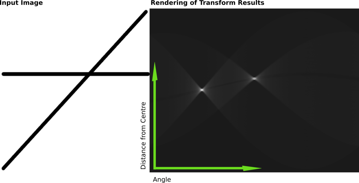*Illustration of the Hough Transform (right figure) for the two black lines in the figure on the left* In our algorithm, we use [this ](https://scikit-image.org/docs/stable/auto_examples/edges/plot_line_hough_transform.html)implementation from scikit-image because it is easier to configure. Also, this library provides a convenient method for selecting local maxima that resemble the lines the most. The OpenCV [implementation](https://opencv24-python-tutorials.readthedocs.io/en/latest/py_tutorials/py_imgproc/py_houghlines/py_houghlines.html) doesn’t have a similar feature. ``` tested_angles = np.linspace(-1.6, 1.6, 410) h, theta, d = transform.hough_line(img_canny, theta=tested_angles) _, angles, dists = transform.hough_line_peaks(h, theta, d) ``` The transform outputs the angles and distances to the found lines. Drawing these lines is a bit trickier than the lines we are used to, so here is an additional snippet of code. ``` plt.figure(figsize=(10, 10)) plt.imshow(img_gray, cmap="gray") x = np.array((0, img_gray.shape[1])) ys = [] for angle, dist in zip(angles, dists): y0, y1 = (dist - x * np.cos(angle)) / np.sin(angle) y = int(np.mean([y0, y1])) ys += [y] plt.plot(x, [y, y]) ys = np.array(ys) plt.axis("off"); ``` The found distance is the hypotenuse and the position of the line along the y-axis is the cathetus, so we divide the distance value by the sine of the resulting angle. As a result of running this code, you will see the following: 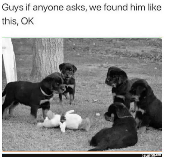Our algorithm found all the necessary lines! The border of our app watermark at the very bottom is also detected. **Step 4. Classification of lines** Finally, we need to determine which is the bottom line and which is the top one while also removing unnecessary lines, such as the one above the black bar. *Final result* To solve this problem, we added a check of the areas above and below the found lines. Since we work with memes and their captions, we expect the background outside the picture to be white and the text on it to be black. Or vice versa: black background and white letters. Therefore, our algorithm is based on checking the percentage of white and black pixels in the separated areas. ``` props = { "white_limit": 230, "black_limit": 35, "percent_limit": 0.8 } areas_h = [] for y in ys: percent_up = np.sum((img[:y] > props['white_limit']) + (img[:y] < props['black_limit'])) / (y * img.shape[1] * 3) percent_down = np.sum((img[y:] > props['white_limit']) + (img[y:] < props['black_limit'])) / ((img.shape[0] - y) * img.shape[1] * 3) areas_h += [-1 * (percent_up > props['percent_limit']) + (percent_down > props['percent_limit']) * 1] ``` In this approach, we used 3 variables: - white_limit is the lower limit for defining the white color. All pixels with a value in the range (230; 256) will be considered white. - black_limit is the upper limit for defining the black color. All pixels with a value in the range (0; 35) will be considered black. - percent_limit is the minimum percentage of white/black pixels in the area at which the area will be considered as background with text. In addition, the comparison takes place in each color channel independently, which is a general enough condition that allows you to correctly handle rare exceptions. ```cut_threshold = 0.6 y0 = np.max(ys[areas_h == -1]) if y0 > cut_threshold * img.shape[0]: y0 = 0 y1 = np.min(ys[areas_h == 1]) if y1 < (1 - cut_threshold) * img.shape[0]: y1 = img.shape[0] ``` The following few lines of code select the lowest line among the upper limits and the top line among the lower limits. We also added a condition for the size of the chosen area. If the resulting vertical line cuts off more than 60% of the image height, we consider it an error and return the top or bottom border of the original image. This parameter is chosen based on the assumption of the area occupied by the meme image. The final algorithm, which you can find in the Functions section here, also includes finding and adjusting vertical borders, allowing you to remove frames on the sides of the image. **What’s next?** To improve results, you need to learn how to measure quality, and for that, you need markup. If you want to create a training dataset, our algorithm will make your manual markup easier, allowing you to collect the required number of examples faster. To generalize our approach for more cases, you can replace the background color check in the algorithm with a monochrome review. This will allow the method to be used regardless of the background color.